Attention Maps#
Attention maps let you overlay a per-sample scalar score on top of the ECG trace. A typical use-case is visualising the output of a neural network: which time steps did the model attend to when it produced a particular prediction?
This page shows how to build attention data, choose the right map style, and use the built-in annotation helpers.
Setup#
import wfdb
import numpy as np
import pandas as pd
import pmecg

record = wfdb.rdrecord('00001_hr', pn_dir='ptb-xl/1.0.3/records500/00000/')
ecg_df = pd.DataFrame(record.p_signal, columns=record.sig_name)
fs = record.fs

# PTB-XL uses uppercase AVR/AVL/AVF; map them to canonical names (aVR/aVL/aVF).
leads_map = pmecg.LeadsMap(aVR='AVR', aVL='AVL', aVF='AVF')

n_samples = len(ecg_df)
Creating Attention Data#
Attention data must be a pandas.DataFrame whose columns match the ECG lead
names (or a (array, lead_names) tuple — the same formats accepted by
ECGPlotter.plot).
Here we simulate model attention using a sine wave on two leads. Oscillating between −1 and +1 makes this a natural example of signed attention — positive values mean the model attended strongly in one direction, negative in the other.
period = n_samples / 3  # one cycle every third of the recording → 3 full cycles
t = np.arange(n_samples)

# When the attention DataFrame has more than one column, every ECG lead must
# be present. We start from a zero-filled DataFrame (one column per lead) and
# then assign values only to the two leads of interest.
attention_df = pd.DataFrame(0.0, index=ecg_df.index, columns=ecg_df.columns)
attention_df['II'] = np.sin(2 * np.pi * t / period)            # full range [-1, 1]
attention_df['V5'] = np.sin(2 * np.pi * t / period + np.pi)   # same shape, phase-shifted
All three map types below accept this DataFrame directly.
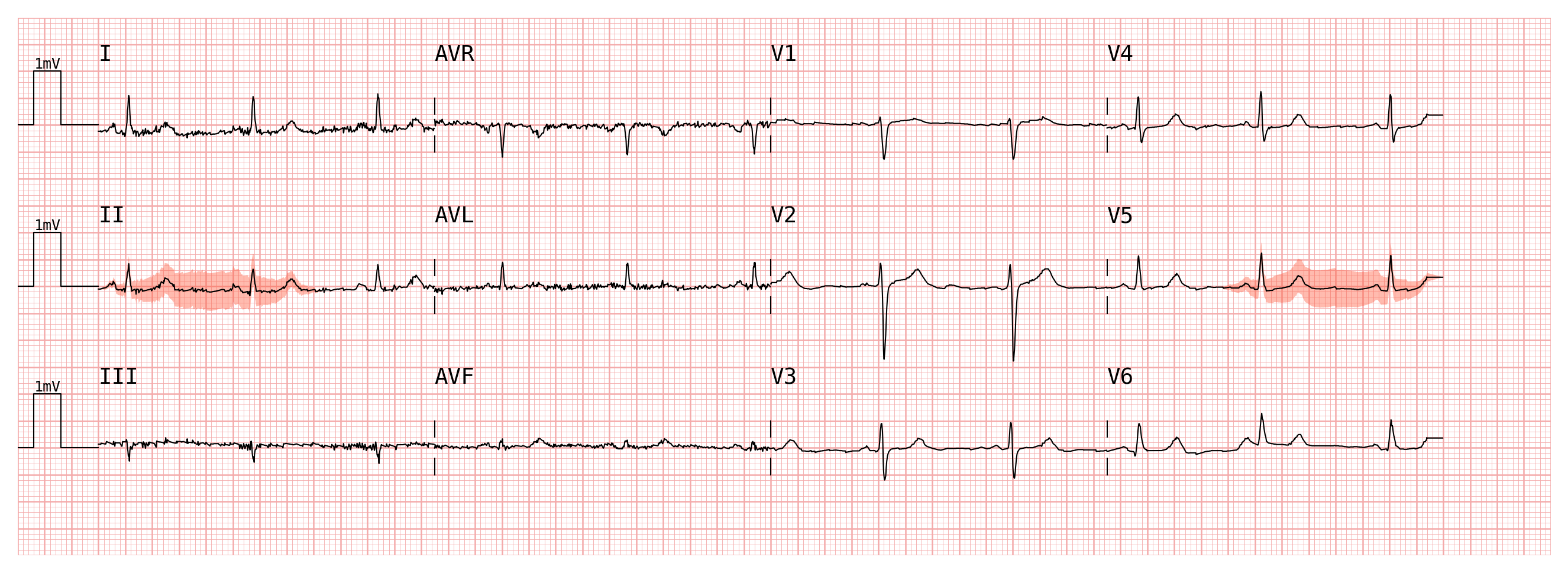
Interval Attention Map#
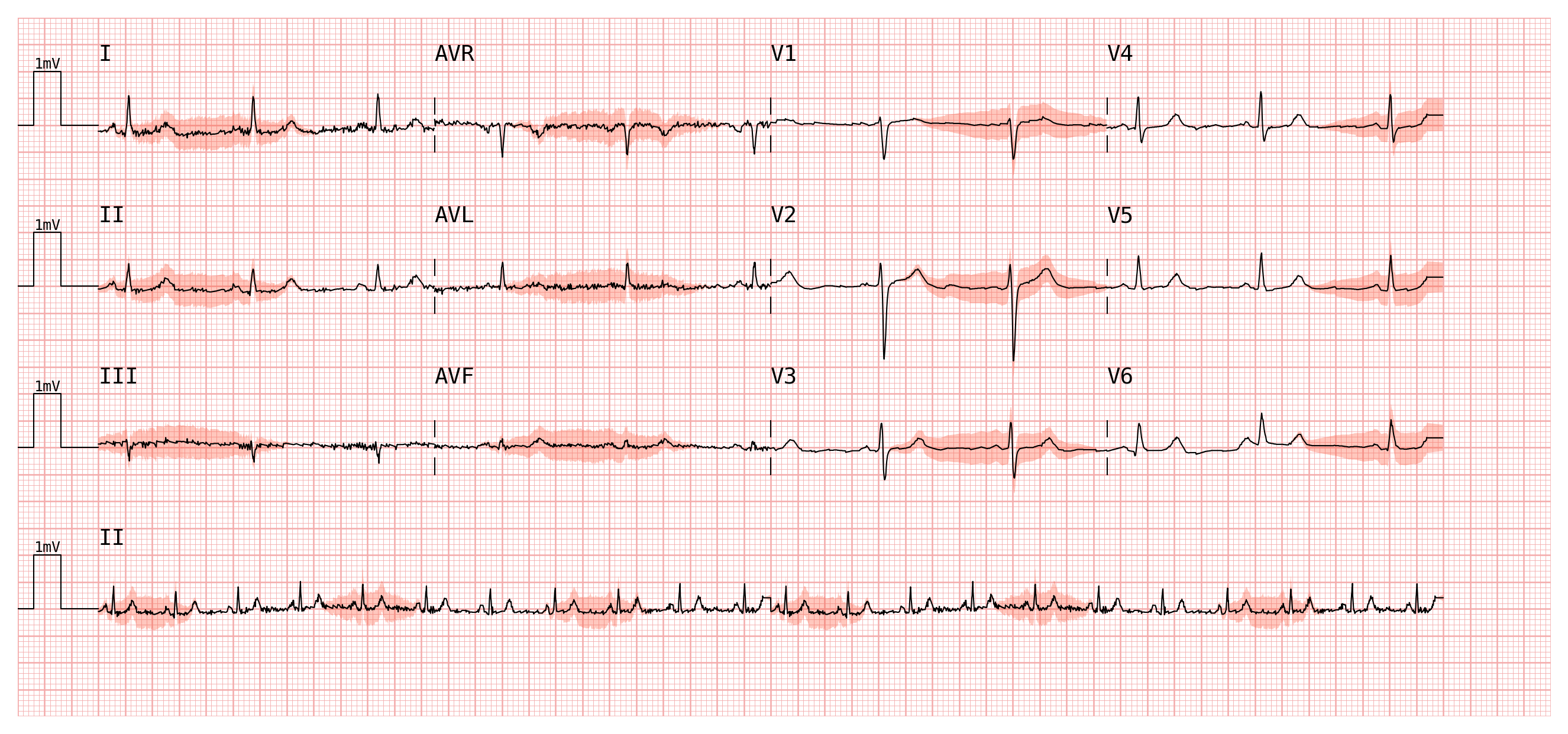
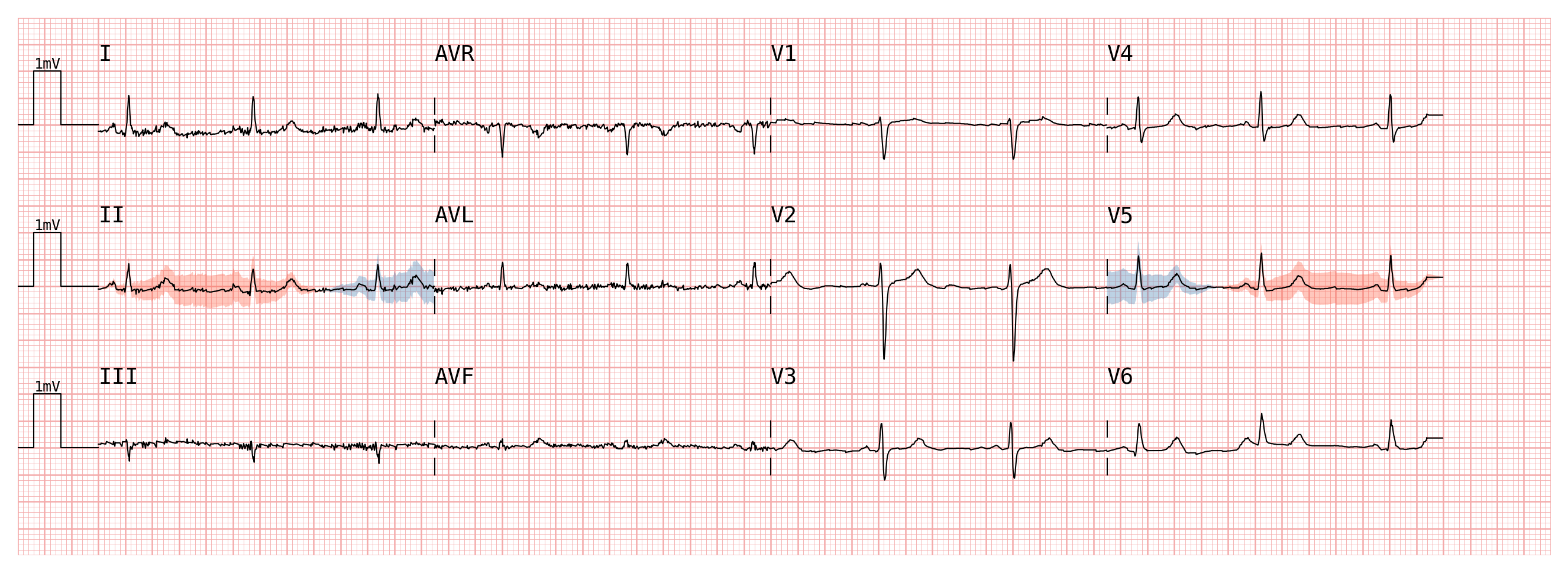
IntervalAttentionMap draws a band around the ECG trace whose half-width
scales with the attention magnitude. This is the least visually intrusive style
— it leaves the trace itself untouched.
# polarity='signed' → values may be negative or positive.
# color=(negative_color, positive_color) — two strings, one per sign.
interval_map = pmecg.IntervalAttentionMap(
    attention_df,
    polarity='signed',
    color=('steelblue', 'tomato'),   # blue for negative, red for positive
    max_attention_mV=0.3,            # band half-width at full attention strength
    alpha=0.4,
    smoothing_window=4,             # light smoothing to reduce visual noise
)

plotter = pmecg.ECGPlotter(grid_mode='cm')
fig = plotter.plot(
    ecg_df,
    configuration=pmecg.template_factory('4x3', ecg_df, leads_map=leads_map),
    sampling_frequency=fs,
    attention_map=interval_map,
    show=True,
)
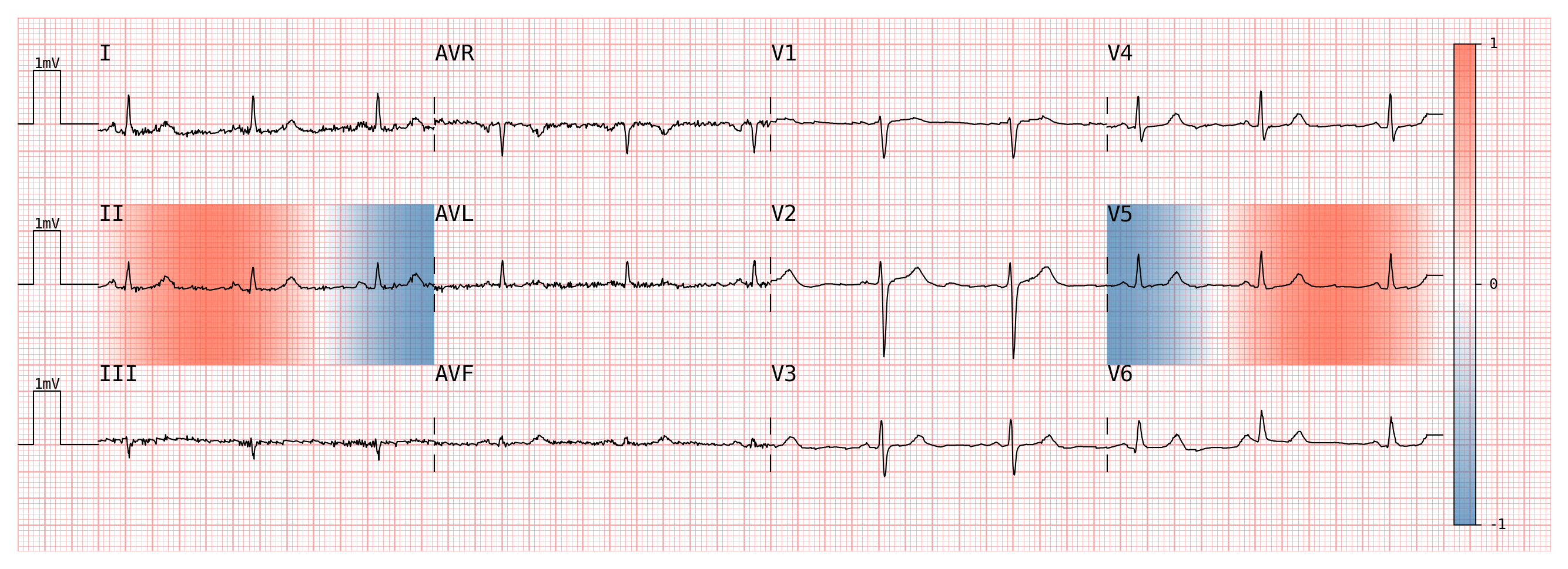
Background Attention Map#
BackgroundAttentionMap fills the full height of each row with a
semi-transparent color block. The opacity scales with the attention magnitude,
so high-attention regions are visually dominant.
# show_colormap=True (default) adds a vertical color scale on the right margin.
# The plotter automatically widens the figure to preserve the ECG trace area.
background_map = pmecg.BackgroundAttentionMap(
    attention_df,
    polarity='signed',
    color=('steelblue', 'tomato'),
    show_colormap=True,
)

fig = plotter.plot(
    ecg_df,
    configuration=pmecg.template_factory('4x3', ecg_df, leads_map=leads_map),
    sampling_frequency=fs,
    attention_map=background_map,
    show=True,
)
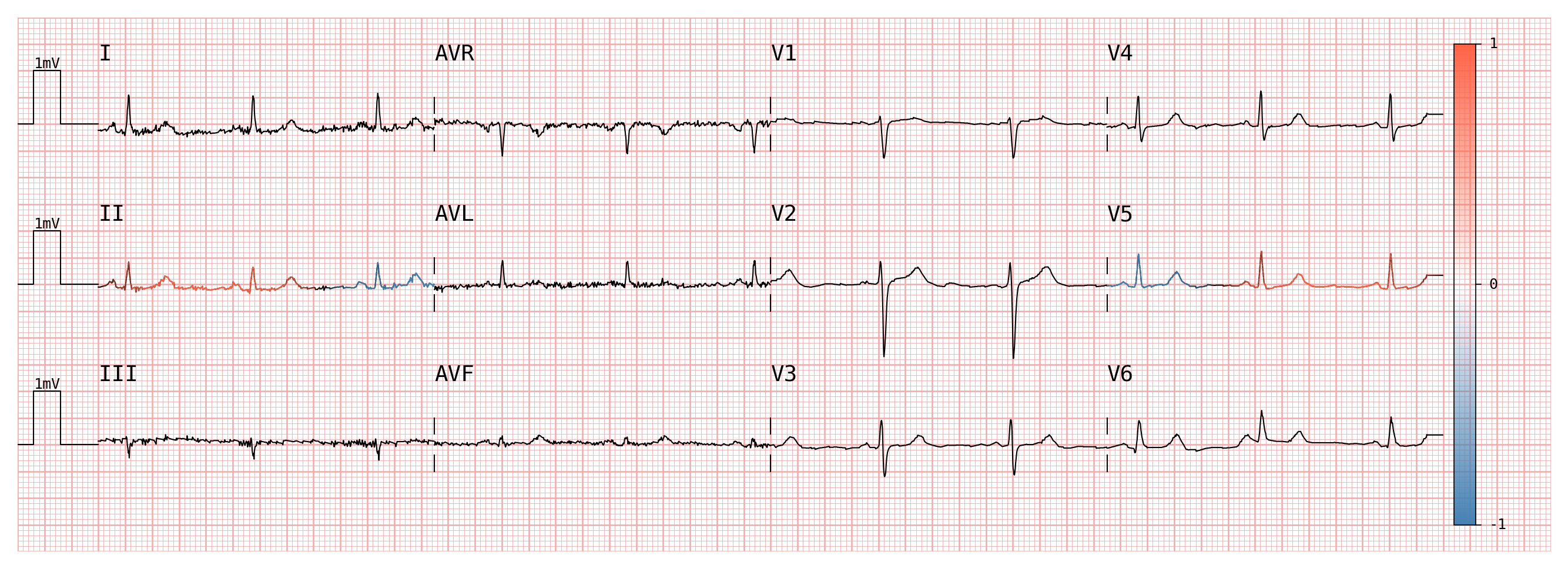
Line Color Attention Map#
LineColorAttentionMap recolors the ECG trace itself: each segment of the
line is assigned a color whose opacity reflects the local attention value.
Segments with zero attention are invisible, so the original black trace
disappears where the model did not attend.
line_map = pmecg.LineColorAttentionMap(
    attention_df,
    polarity='signed',
    color=('steelblue', 'tomato'),
    show_colormap=True,
)

fig = plotter.plot(
    ecg_df,
    configuration=pmecg.template_factory('4x3', ecg_df, leads_map=leads_map),
    sampling_frequency=fs,
    attention_map=line_map,
    show=True,
)
Unipolar (Positive) Attention#
When attention scores are strictly non-negative — for example, the output of a
softmax or a ReLU — use polarity='positive'. The 'positive' polarity
requires that all values are ≥ 0 and that at least one value is > 0. If
your raw scores can go negative, clip them first.
# Clip the signed sine wave to [0, 1] before passing it to the map.
# Any sample where the original value was negative will now have zero attention.
positive_attention_df = attention_df.clip(lower=0.0, upper=1.0)

# polarity='positive' → color is a single string, not a tuple.
interval_map_positive = pmecg.IntervalAttentionMap(
    positive_attention_df,
    polarity='positive',
    color='tomato',
    max_attention_mV=0.35,
    alpha=0.5,
    smoothing_window=4,
)

fig = plotter.plot(
    ecg_df,
    configuration=pmecg.template_factory('4x3', ecg_df, leads_map=leads_map),
    sampling_frequency=fs,
    attention_map=interval_map_positive,
    show=True,
)
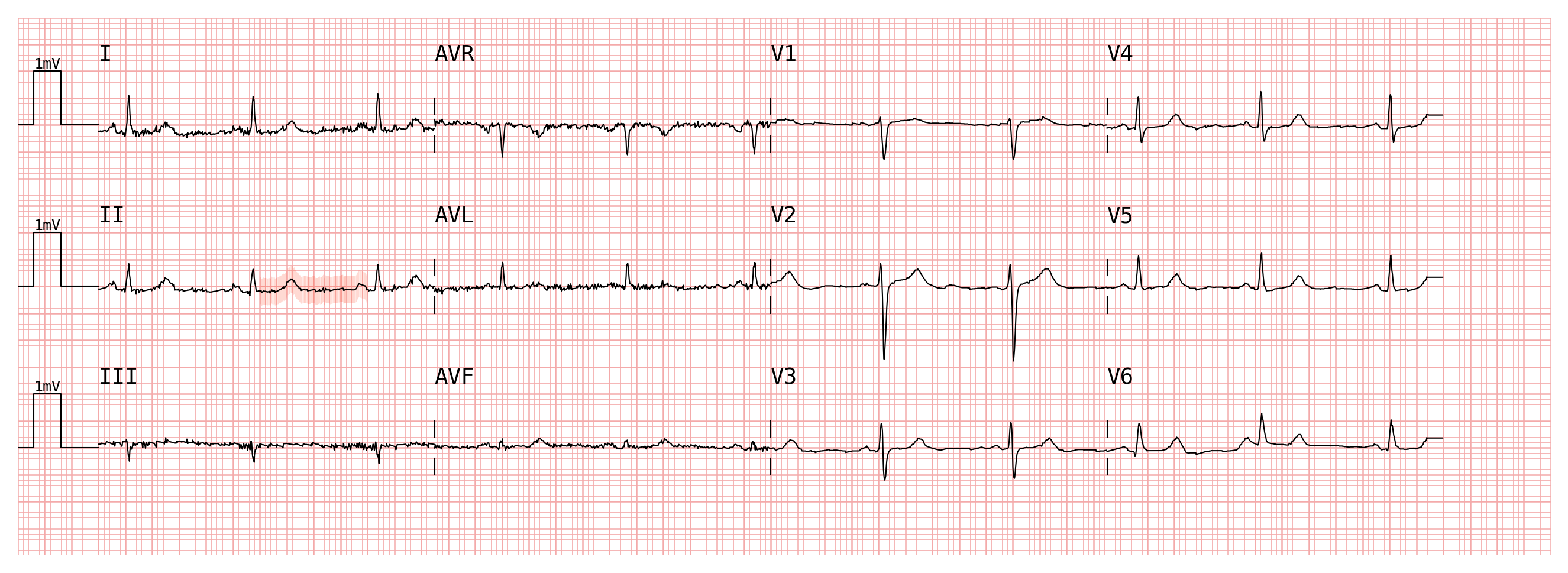
Using attention_map_from_time_annotations#
Building a full attention array manually can be tedious when you only need to
highlight a handful of time windows. attention_map_from_time_annotations
accepts sparse annotations expressed in seconds and fills in the rest with
zeros.
Each annotation is a dict with two keys:
Key |
Type |
Meaning |
|---|---|---|
|
|
Half-open interval in seconds |
|
|
Scalar score to assign to every sample in the window |
# Highlight two suspicious windows on lead II and one on V2.
# All other leads and time steps are filled with 0 automatically.
annotation_map_df = pmecg.attention_map_from_time_annotations(
    ecg_df,
    fs,                             # sampling frequency, needed to convert seconds → indices
    II=[
        {'time_range': (1.2, 2.0), 'attention_value': 0.9},   # first window, strong attention
        {'time_range': (6.5, 7.5), 'attention_value': 0.5},   # second window, moderate
    ],
    V2=[
        {'time_range': (3.0, 4.5), 'attention_value': 0.75},
    ],
)

# The result is a plain DataFrame — inspect it like any other attention input.
print(annotation_map_df.describe())
            I           II     III     AVR     AVL     AVF      V1  \
count  5000.0  5000.000000  5000.0  5000.0  5000.0  5000.0  5000.0
mean      0.0     0.122000     0.0     0.0     0.0     0.0     0.0
std       0.0     0.273735     0.0     0.0     0.0     0.0     0.0
min       0.0     0.000000     0.0     0.0     0.0     0.0     0.0
25%       0.0     0.000000     0.0     0.0     0.0     0.0     0.0
50%       0.0     0.000000     0.0     0.0     0.0     0.0     0.0
75%       0.0     0.000000     0.0     0.0     0.0     0.0     0.0
max       0.0     0.900000     0.0     0.0     0.0     0.0     0.0

               V2      V3      V4      V5      V6
count  5000.00000  5000.0  5000.0  5000.0  5000.0
mean      0.11250     0.0     0.0     0.0     0.0
std       0.26783     0.0     0.0     0.0     0.0
min       0.00000     0.0     0.0     0.0     0.0
25%       0.00000     0.0     0.0     0.0     0.0
50%       0.00000     0.0     0.0     0.0     0.0
75%       0.00000     0.0     0.0     0.0     0.0
max       0.75000     0.0     0.0     0.0     0.0
Pass the DataFrame to any attention map class:
annotation_interval = pmecg.IntervalAttentionMap(
    annotation_map_df,
    polarity='positive',   # all values are 0 or positive by construction
    color='tomato',
    smoothing_window=4,
)

fig = plotter.plot(
    ecg_df,
    configuration=pmecg.template_factory('4x3', ecg_df, leads_map=leads_map),
    sampling_frequency=fs,
    attention_map=annotation_interval,
    show=True,
)
Tip
If you prefer to annotate by sample index rather than seconds (e.g. when
working with pre-segmented windows), use
pmecg.attention_map_from_indices_annotations with index_range instead of
time_range. The call signature is otherwise identical.
Rhythm Strip Attention#
When rhythm_strips is used together with an attention map, rhythm strip rows are
rendered without an attention overlay by default. To show attention on a
rhythm strip, pass rhythm_strips_attention to the attention map constructor.
The rhythm strip attention data is scaled with the same global scale factor as
data, so colors are directly comparable between the main layout rows and the
rhythm strip rows. The rhythm strip data may have a different number of samples than data —
a common case is a rhythm strip that shows more of the recording (e.g. double
length at half speed).
Any rhythm strip whose name is not present in rhythm_strips_attention is
rendered without an overlay; rhythm strips that are present receive the matching
attention array.
# ecg_df, fs, and plotter are defined in the Setup section above.

# Build a positive attention array for the main layout (all 12 leads).
positive_attention_df = pd.DataFrame(
    np.clip(np.sin(2 * np.pi * np.arange(n_samples)[:, None] / (n_samples / 3) + np.arange(12) * 0.2), 0, None),
    columns=ecg_df.columns,
)

# The rhythm strip (II) shows the recording twice at half speed.
ii_values = ecg_df['II'].to_numpy()
rhythm_strip_signal = np.concatenate([ii_values, ii_values])
rhythm_strip_df = pd.DataFrame({'II': rhythm_strip_signal})

# Build rhythm strip attention at the doubled length by concatenating lead II attention mask to itself.
rhythm_strip_attention_df = pd.concat(
    [positive_attention_df[['II']], positive_attention_df[['II']]],
    axis=0,
    ignore_index=True
)

interval_map_with_rhythm_strip = pmecg.IntervalAttentionMap(
    positive_attention_df,
    polarity='positive',
    color='tomato',
    max_attention_mV=0.3,
    alpha=0.4,
    rhythm_strips_attention=rhythm_strip_attention_df,
)

fig = plotter.plot(
    ecg_df,
    configuration=pmecg.template_factory('4x3', ecg_df, leads_map=leads_map),
    sampling_frequency=fs,
    attention_map=interval_map_with_rhythm_strip,
    rhythm_strips=pmecg.RhythmStripsConfig(ecg_data=rhythm_strip_df, speed=plotter.speed / 2),
    show=True,
)