Advanced configurations

In the basic usage, configuration is a list[list[str] | str]: each inner list is a row, and each string names a lead column. When a row contains n leads, pmecg splits the recording into n equal-length chunks and assigns one chunk to each lead in order. A bare string (instead of a sublist) produces a full-width rhythm strip spanning the entire recording.

This default works well for standard layouts, but two common situations require finer control:

1. Unequal segment lengths. You may want one lead in a row to cover a short diagnostic window (e.g. 0.5 s to zoom in on a P-wave) while another covers most of the recording. Equal splitting via configuration templates cannot express this.

2. Asynchronous plots. Suppose all leads were recorded simultaneously for a short window, and you want every row to show exactly that same time interval in the main grid — while a rhythm strip at the bottom spans a much longer duration. With equal splitting the rhythm strip would be cut to the same length as the main rows, losing the extra context.

In both cases, replace lead name strings with LeadSegment objects. A LeadSegment carries an explicit start and end sample index alongside the lead name, giving you full control over which slice of the signal each cell displays:

from pmecg.types import LeadSegment

LeadSegment(lead='II', start=0, end=2500)   # first 5 s at 500 Hz

The sections below show one example for each scenario.

---

1. Leads with Custom Durations

By default, when a row contains multiple leads, the recording is divided into equal segments — each lead gets the same slice of time. LeadSegment objects let you override this by specifying an explicit start and end sample index for every lead independently.

This is useful when you want to zoom in on a particular interval of a specific lead, or when leads were acquired at different times and their meaningful sections do not align to equal partitions.

Each LeadSegment takes three arguments:

Argument	Type	Description
lead	str	Column name in the input data
start	int	First sample (inclusive)
end	int	Last sample (exclusive)

For consistent visual output, all rows should produce the same total number of samples. If a row has two leads each spanning 2 500 samples, every other row should also total 5 000 samples so that each row has the same physical width on the page. pmecg will issue a warning if row lengths differ.

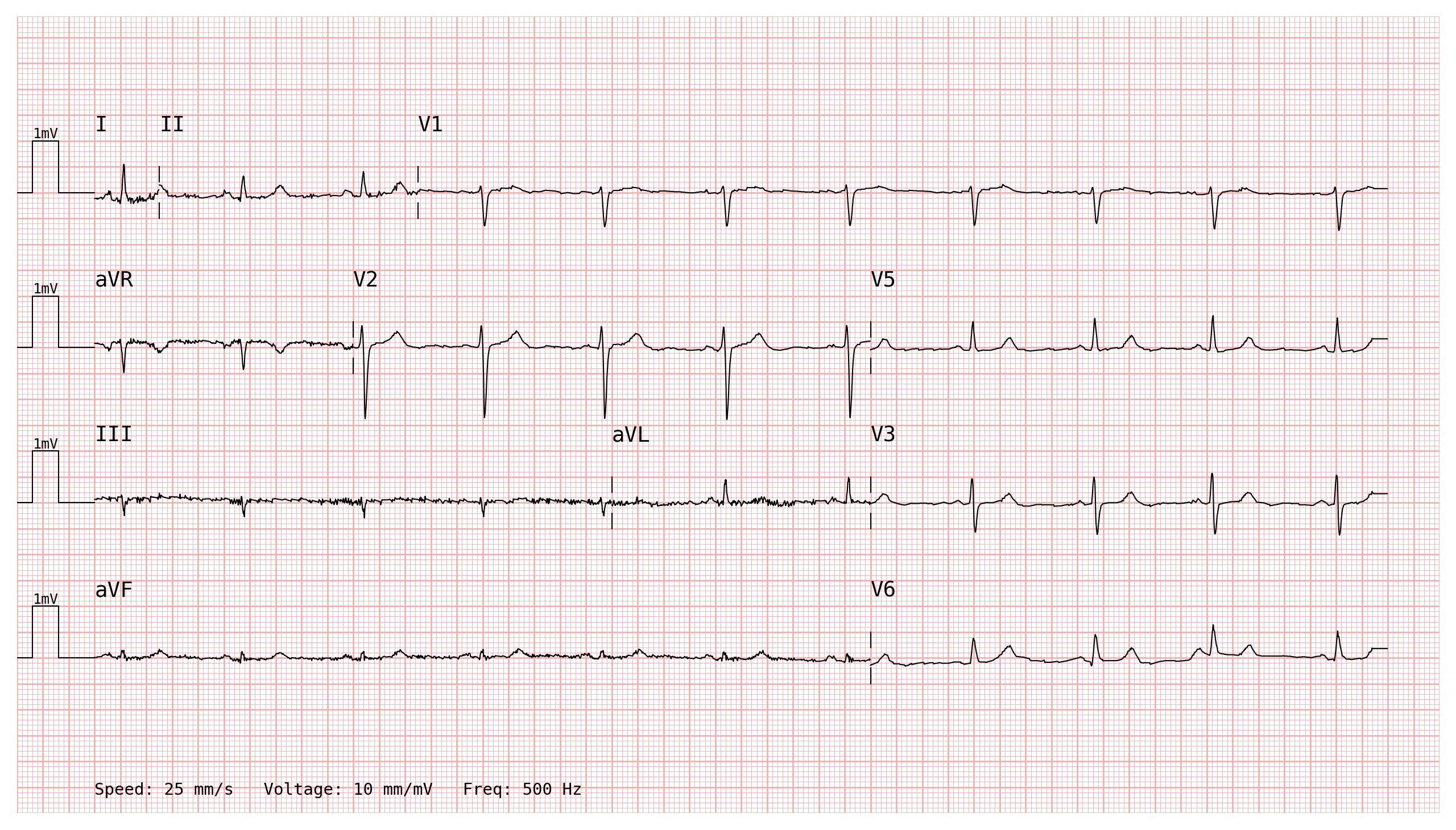
The example below uses fully irregular rows: each row contains a different number of leads, and each lead is allocated a different time window. All rows total the same number of samples — here 5 000 (10 s at 500 Hz) — but how those samples are distributed across leads is entirely up to you.

This layout could represent an annotator’s choice to spend more “page space” on leads or intervals that are diagnostically relevant and less on quieter sections:

import wfdb
import pandas as pd
import numpy as np
import pmecg

record = wfdb.rdrecord('00001_hr', pn_dir='ptb-xl/1.0.3/records500/00000/')
ecg_df = pd.DataFrame(record.p_signal, columns=record.sig_name)
# PTB-XL uses uppercase "AVR"/"AVL"/"AVF"; rename to canonical names
ecg_df = ecg_df.rename(columns={"AVR": "aVR", "AVL": "aVL", "AVF": "aVF"})
fs = record.fs

from pmecg.types import LeadSegment

N = ecg_df.shape[0]  # 5000 samples = 10 s at 500 Hz

# Row 1 — 3 leads with unequal windows (0.5 s | 2 s | 7.5 s)
# e.g. a short glance at the P-wave onset in I, a medium window of II,
# then a long view of V1 covering most of the recording.
row1 = [
    LeadSegment(lead='I',   start=0,    end=250),    # 0.5 s
    LeadSegment(lead='II',  start=250,  end=1250),   # 2.0 s
    LeadSegment(lead='V1',  start=1250, end=N),      # 7.5 s
]

# Row 2 — 3 leads, different split (2 s | 4 s | 4 s)
row2 = [
    LeadSegment(lead='aVR', start=0,    end=1000),   # 2.0 s
    LeadSegment(lead='V2',  start=1000, end=3000),   # 4.0 s
    LeadSegment(lead='V5',  start=3000, end=N),      # 4.0 s
]

# Row 3 — 3 leads, yet another split (4 s | 2 s | 4 s)
row3 = [
    LeadSegment(lead='III', start=0,    end=2000),   # 4.0 s
    LeadSegment(lead='aVL', start=2000, end=3000),   # 2.0 s
    LeadSegment(lead='V3',  start=3000, end=N),      # 4.0 s
]

# Row 4 — only 2 leads (6 s | 4 s)
row4 = [
    LeadSegment(lead='aVF', start=0,    end=3000),   # 6.0 s
    LeadSegment(lead='V6',  start=3000, end=N),      # 4.0 s
]

plotter = pmecg.ECGPlotter(grid_mode='cm', print_information=True)
fig = plotter.plot(
    ecg_df,
    configuration=[row1, row2, row3, row4],
    sampling_frequency=fs,
    show=True,
)

---

2. Asynchronous Rhythm Strip

RhythmStripsConfig accepts its own ecg_data DataFrame and an optional speed, appending one or more full-width rhythm strip rows below the main layout — completely independent of the main configuration’s time range.

Suppose you have recorded:

• 10 seconds for all leads

• 20 seconds for the rhythm strip (here, lead II)

And you want to plot:

• the first 5 seconds of all leads in a 2×6 layout

• the rhythm strip for the entire 20 seconds

You could use the 2x6+1 template, but that produces a synchronous plot sharing one time axis. This means that:

• the first column shows the first half of the signals

• the second column shows the second half of the signals

Instead, use a LeadSegment-based main configuration combined with RhythmStripsConfig carrying its own data:

from pmecg.types import LeadSegment
from pmecg import RhythmStripsConfig

# First 5 s per lead
half = ecg_df.shape[0] // 2

# Rhythm strip: 20 s long — obtained by concatenating lead II with itself.
rhythm_strip_df = pd.concat([ecg_df[['II']], ecg_df[['II']]], ignore_index=True)

# Main rows: 2 leads per row, each showing the first 5 s.
# 2 leads × 2500 samples = 5000 samples per row → 5000/500 Hz × 25 mm/s = 250 mm wide
main_config = [
    [
        LeadSegment(lead='I',   start=0, end=half),
        LeadSegment(lead='V1',  start=0, end=half),
    ],
    [
        LeadSegment(lead='II',  start=0, end=half),
        LeadSegment(lead='V2',  start=0, end=half),
    ],
    [
        LeadSegment(lead='III', start=0, end=half),
        LeadSegment(lead='V3',  start=0, end=half),
    ],
    [
        LeadSegment(lead='aVR', start=0, end=half),
        LeadSegment(lead='V4',  start=0, end=half),
    ],
    [
        LeadSegment(lead='aVL', start=0, end=half),
        LeadSegment(lead='V5',  start=0, end=half),
    ],
    [
        LeadSegment(lead='aVF', start=0, end=half),
        LeadSegment(lead='V6',  start=0, end=half),
    ],
]

# Rhythm strip: 20 s long at half the main speed → 10000/500 Hz × 12.5 mm/s = 250 mm wide.
# The rhythm strip fits in the same page width as the main rows.
rhythm_strips = RhythmStripsConfig(ecg_data=rhythm_strip_df, speed=12.5)

plotter = pmecg.ECGPlotter(grid_mode='cm', speed=25.0, print_information=True)
fig = plotter.plot(
    ecg_df,
    configuration=main_config,
    rhythm_strips=rhythm_strips,
    sampling_frequency=fs,
    show=True,
)

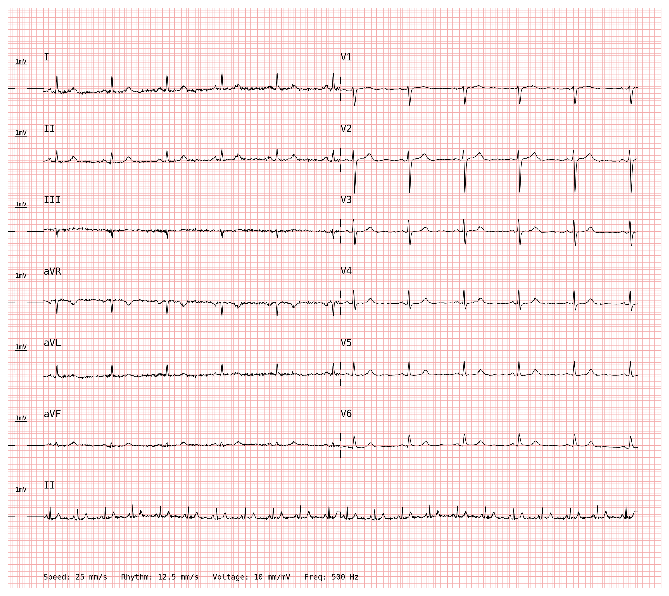
The rhythm strip row carries a Rhythm: 12.5 mm/s annotation when print_information=True, making the different scale immediately visible to the reader.